Realistic Example

A close-to-real-world example of how to use firelight.

First of all, let us get some mock data to visualize. We generate the following tensors:

• input of shape \((B, D, H, W)\), some noisy raw data,

• target of shape \((B, D, H, W)\), the ground truth foreground background segmentation,

• prediction of shape \((B, D, H, W)\), the predicted foreground probability,

• embedding of shape \((B, D, C, H, W)\), a tensor with an additional channel dimension, as for example intermediate activations of a neural network.

import numpy as np
import torch
from skimage.data import binary_blobs
from skimage.filters import gaussian


def get_example_states():
    # generate some toy foreground/background segmentation
    batchsize = 5  # we will only visualize 3 of the 5samples
    size = 64
    target = np.stack([binary_blobs(length=size, n_dim=3, blob_size_fraction=0.25, volume_fraction=0.5, seed=i)
                       for i in range(batchsize)], axis=0).astype(np.float32)

    # generate toy raw data as noisy target
    sigma = 0.5
    input = target + np.random.normal(loc=0, scale=sigma, size=target.shape)

    # compute mock prediction as gaussian smoothing of input data
    prediction = np.stack([gaussian(sample, sigma=3, truncate=2.0) for sample in input], axis=0)
    prediction = 10 * (prediction - 0.5)

    # compute mock embedding (if you need an image with channels for testing)
    embedding = np.random.randn(prediction.shape[0], 16, *(prediction.shape[1:]))

    # put input, target, prediction in dictionary, convert to torch.Tensor, add dimensionality labels ('specs')
    state_dict = {
        'input': (torch.Tensor(input).float(), 'BDHW'),  # Dimensions are B, D, H, W = Batch, Depth, Height, Width
        'target': (torch.Tensor(target).float(), 'BDHW'),
        'prediction': (torch.Tensor(prediction).float(), 'BDHW'),
        'embedding': (torch.Tensor(embedding).float(), 'BCDHW'),
    }
    return state_dict


# Get the example state dictionary, containing the input, target, prediction.
states = get_example_states()

for name, (tensor, spec) in states.items():
    print(f'{name}: shape {tensor.shape}, spec {spec}')

Out:

input: shape torch.Size([5, 64, 64, 64]), spec BDHW
target: shape torch.Size([5, 64, 64, 64]), spec BDHW
prediction: shape torch.Size([5, 64, 64, 64]), spec BDHW
embedding: shape torch.Size([5, 16, 64, 64, 64]), spec BCDHW

The best way to construct a complex visualizer to show all the tensors in a structured manner is to use a configuration file.

We will use the following one:

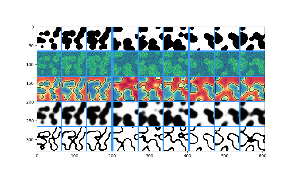
RowVisualizer: # stack the outputs of child visualizers as rows of an image grid
  input_mapping:
    global: [B: ':3', D: '0:9:3'] # Show only 3 samples in each batch ('B'), and some slices along depth ('D').
    prediction: [C: '0']  # Show only the first channel of the prediction

  pad_value: [0.2, 0.6, 1.0] # RGB color of separating lines
  pad_width: {B: 6, H: 0, W: 0, rest: 3} # Padding for batch ('B'), height ('H'), width ('W') and other dimensions.

  visualizers:
    # First row: Ground truth
    - IdentityVisualizer:
        input: 'target' # show the target

    # Second row: Raw input
    - IdentityVisualizer:
        input: ['input', C: '0'] # Show the first channel ('C') of the input.
        cmap: viridis  # Name of a matplotlib colormap.

    # Third row: Prediction with segmentation boarders on top.
    - OverlayVisualizer:
        visualizers:
          - CrackedEdgeVisualizer: # Show borders of target segmentation
              input_mapping:
                segmentation: 'target'
              width: 2
              opacity: 0.7 # Make output only partially opaque.
          - IdentityVisualizer: # prediction
              input_mapping:
                tensor: 'prediction'
              cmap: Spectral

    # Fourth row: Foreground probability, calculated by sigmoid on prediction
    - IdentityVisualizer:
        input_mapping: # the input to the visualizer can also be specified as a dict under the key 'input mapping'.
          tensor: ['prediction', pre: 'sigmoid'] # Apply sigmoid function from torch.nn.functional before visualize.
        value_range: [0, 1] # Scale such that 0 is white and 1 is black. If not specified, whole range is used.

    # Fifth row: Visualize where norm of prediction is smaller than 2
    - ThresholdVisualizer:
        input_mapping:
          tensor:
            NormVisualizer: # Use the output of NormVisualizer as the input to ThresholdVisualizer
              input: 'prediction'
              colorize: False
        threshold: 2
        mode: 'smaller'

Lets load the file and construct the visualizer using get_visualizer:

from firelight import get_visualizer
import matplotlib.pyplot as plt

# Load the visualizer, passing the path to the config file. This happens only once, at the start of training.
visualizer = get_visualizer('example_config_0.yml')

Out:

/home/docs/checkouts/readthedocs.org/user_builds/firelight/checkouts/latest/firelight/utils/io_utils.py:22: YAMLLoadWarning: calling yaml.load() without Loader=... is deprecated, as the default Loader is unsafe. Please read https://msg.pyyaml.org/load for full details.
  readict = yaml.load(f)
[+][2019-11-11 14:56:22,818][VISUALIZATION] Parsing RowVisualizer
[+][2019-11-11 14:56:22,818][VISUALIZATION] Parsing   IdentityVisualizer
[+][2019-11-11 14:56:22,818][VISUALIZATION] Parsing   IdentityVisualizer
[+][2019-11-11 14:56:22,818][VISUALIZATION] Parsing   OverlayVisualizer
[+][2019-11-11 14:56:22,818][VISUALIZATION] Parsing     CrackedEdgeVisualizer
[+][2019-11-11 14:56:22,825][VISUALIZATION] Parsing     IdentityVisualizer
[+][2019-11-11 14:56:22,826][VISUALIZATION] Parsing   IdentityVisualizer
[+][2019-11-11 14:56:22,826][VISUALIZATION] Parsing   ThresholdVisualizer
[+][2019-11-11 14:56:22,826][VISUALIZATION] Parsing     NormVisualizer

Now we can finally apply it on out mock tensors to get the visualization

# Call the visualizer.
image_grid = visualizer(**states)

# Log your image however you want.
plt.figure(figsize=(10, 6))
plt.imshow(image_grid.numpy())